Ps1. 如何新增 R Script:File > New File > R Script
Ps2. 如何安裝 RStudio,參考此頁:Setup instructions
Ps3. 此為筆記,其他細節請參考此頁:Introduction to R - Part 1

(點這裡看放大圖片)
R 裡面可以設定 variable or object,用 <- 設定,可以是數字或是文字。
在 R 語言裡面 ## 可用作註釋,等於 C++ 裡面的 //。(紫色框框裡為打在 R Script 或是 Console 裡的指令,白色框框裡面為跑指令後在 Console 裡出現的結果。)
例如我們可以指定 variables: x1, x2, y
把 x1 指定為 3
|
x1 <- 3 x1 |
| [1] 3 |
如果指定為一個算式的話,就有計算的功能。
|
x2 <- 1 + 2 ## 計算 1 + 2 x2 |
| [1] 3 |
也可以把 variable 或 object 設為文字。
|
y <- "Hello" y |
| [1] "Hello" |
以上三個可以寫在 R script 裡,然後按 "Run",或是在 Console 裡面打 x1, x2, y 跑出來,也可以直接全部打在 Console 的地方。在 Console 打 x1 和 x2 都會出現 [1] 3,打 y 會出現 [1] "Hello"。
R 裡面有很多內建檔案可以拿來練習,例如 mtcars。
在 Console 打入下面的語言可以查詢,會顯示在左上角的視窗。
library()
查看有什麼可用的 packages
data()
叫出 R 裡面的 data, 可以是內建的檔案。
Ex: data(mtcars)
(ps. mtcars 為 R 裡面內建的檔案資料。)
Functions in R
rm()
remove, 用來移除 variables
Ex: rm(x1)
ls()
list objects, 列出所有的 variables
| ls(mtcars) |
|
[1] "am" "carb" "cyl" "disp" "drat" "gear" "hp" "mpg" "qsec" [10] "vs" "wt" |
rename()
改變 variable 的名稱
View()
觀看叫出的 data,會顯示在 script 的那個視窗裡。
Ex: View(mtcars)
str()
觀看檔案資料的細節
| str(mtcars) |
|
'data.frame': 32 obs. of 11 variables: $ mpg : num 21 21 22.8 21.4 18.7 18.1 14.3 24.4 22.8 19.2 ... $ cyl : num 6 6 4 6 8 6 8 4 4 6 ... $ disp: num 160 160 108 258 360 ... $ hp : num 110 110 93 110 175 105 245 62 95 123 ... $ drat: num 3.9 3.9 3.85 3.08 3.15 2.76 3.21 3.69 3.92 ... $ wt : num 2.62 2.88 2.32 3.21 3.44 ... $ qsec: num 16.5 17 18.6 19.4 17 ... $ vs : num 0 0 1 1 0 1 0 1 1 1 ... $ am : num 1 1 1 0 0 0 0 0 0 0 ... $ gear: num 4 4 4 3 3 3 3 4 4 4 ... $ carb: num 4 4 1 1 2 1 4 2 2 4 ... |
每個 variable 裡面的數值或是樣式叫做觀察值 observations,例如在 mtcars 裡面所有的 variables 的觀察值都是數字,但觀察值也可以是 character 或是 factor。
要知道某個 variables (裡的觀察值)是哪種格式(數字, 文字或 factor)可以用 class() 的功能去查看。
class()
檢視某個 variable 的格式
| class(mtcars$cyl) |
| [1] "numeric" |
levels()
檢視某個 variable 裡面的觀察值(observations)有哪些,觀察值的格式必須是 factor 才能顯示出來,如果是數字就會顯示 NULL。
| levels(mtcars$cyl) |
| NULL |
在執行某些指令時,會需要 variables 的格式是 factor,這時候就可以用 factor() 的功能把它轉成 factor。
factor()
把非 factor 的 variables 轉換成 factor
| factor(mtcars$cyl) |
|
[1] 6 6 4 6 8 6 8 4 4 6 6 8 8 8 8 8 8 4 4 4 4 8 8 8 8 [26] 4 4 4 8 6 8 4 Levels: 4 6 8 |
如果 variable 是數字的話,是沒有 levels 的,需要轉成 factor 才有。Levels 是指那個 variable 裡面有哪些 categories,例如把 cyl 轉成 factor 的話,就有 4, 6, 8 三種。
下面用 class() 去檢視,是否真的把原本是數字的 cyl 轉成 factor。
| class(factor(mtcars$cyl)) |
| [1] "factor" |
也可以用 levels() 去檢視,轉成 factor 後就不會像上面出現 NULL。
| levels(factor(mtcars$cyl)) |
| [1] "4" "6" "8" |
summary()
觀看檔案資料的總節
| summary(mtcars) |
|
mpg cyl disp Min. :10.40 Min. :4.000 Min. : 71.1 1st Qu.:15.43 1st Qu.:4.000 1st Qu.:120.8 Median :19.20 Median :6.000 Median :196.3 Mean :20.09 Mean :6.188 Mean :230.7 3rd Qu.:22.80 3rd Qu.:8.000 3rd Qu.:326.0 Max. :33.90 Max. :8.000 Max. :472.0 hp drat wt Min. : 52.0 Min. :2.760 Min. :1.513 1st Qu.: 96.5 1st Qu.:3.080 1st Qu.:2.581 Median :123.0 Median :3.695 Median :3.325 Mean :146.7 Mean :3.597 Mean :3.217 3rd Qu.:180.0 3rd Qu.:3.920 3rd Qu.:3.610 Max. :335.0 Max. :4.930 Max. :5.424 |
dim()
dimension, # of row and column.
| dim(mtcars) |
| [1] 32 11 |
(ps. row = 32, column = 11)
nrow()
# of rows
| nrow(mtcars) |
| [1] 32 |
ncol()
# of columns
| ncol(mtcars) |
| [1] 11 |
head()
列出檔案資料中的前幾項
head(x, #)
x = object or dataframe
n = number, # of elements
列出 mtcars 的前十個 variables 的資料
| head(mtcars, 10) |
|
mpg cyl disp hp drat wt qsec vs Mazda RX4 21.0 6 160.0 110 3.90 2.620 16.46 0 Mazda RX4 Wag 21.0 6 160.0 110 3.90 2.875 17.02 0 Datsun 710 22.8 4 108.0 93 3.85 2.320 18.61 1 Hornet 4 Drive 21.4 6 258.0 110 3.08 3.215 19.44 1 Hornet Sportabout 18.7 8 360.0 175 3.15 3.440 17.02 0 Valiant 18.1 6 225.0 105 2.76 3.460 20.22 1 Duster 360 14.3 8 360.0 245 3.21 3.570 15.84 0 Merc 240D 24.4 4 146.7 62 3.69 3.190 20.00 1 Merc 230 22.8 4 140.8 95 3.92 3.150 22.90 1 Merc 280 19.2 6 167.6 123 3.92 3.440 18.30 1 |
查詢檔案資料的某個 variable:dataframeName$VariableName
例如 dataframe = mtcars, variable = mpg 的話,就是這樣:
|
z <- mtcars$mpg z |
|
[1] 21.0 21.0 22.8 21.4 18.7 18.1 14.3 24.4 22.8 19.2 17.8 16.4 [13] 17.3 15.2 10.4 10.4 14.7 32.4 30.4 33.9 21.5 15.5 15.2 13.3 [25] 19.2 27.3 26.0 30.4 15.8 19.7 15.0 21.4 |
會叫出 mtcars 檔案裡的 mpg
median(dataframe$variable)
找出檔案中某個 variable 的中間值
例如找出 mtcars 檔案裡 mpg 的 median (中間值)
dataframe = mtcars, variable = mpg
| median(mtcars$mpg) |
| [1] 19.2 |
max(dataframe$variable)
找出檔案資料裡某個 variable 的最大值
| max(mtcars$mpg) |
| [1] 33.9 |
min(dataframe$variable)
找出檔案資料裡某個 variable 的最小值
mean()
算出檔案中某個 variable 的平均值 mean value
| mean(mtcars$mpg) |
| [1] 20.09062 |
算出 mtcars 裡的 mpg 的 mean value (平均值)
sd()
算出 standard deviation
| sd(mtcars$mpg) |
| [1] 6.026948 |
sapply(dataframe, function)
算出檔案裡的所有 variables 的指定數據。
例如算出 mtcars 裡面所有 variables 的平均值
dataframe = mtcars, function = mean
| sapply(mtcars, mean) |
|
mpg cyl disp hp drat wt 20.090625 6.187500 230.721875 146.687500 3.596563 3.217250 qsec vs am gear carb 17.848750 0.437500 0.406250 3.687500 2.812500 |
quantile(x, probs = )
在檔案資料中,分佈圖(distribution)中某些比例的數值。
x = data values, or dataframe$variable
例如找出 mtcars 裡的 mpg 數值裡的第 50% (50th percentile)。
| quantile(mtcars$mpg, prob = 0.5) |
|
50% 6 |
quantile(x, probs = c())
在檔案資料中,分佈圖(distribution)中某些比例的數值。
x = data values, or dataframe$variable
例如找出第 0%, 25% 和第 75% 的值就是:probs = c(0, 0.25, 0.75)
## value at 0-th (0%), 25-th (25%) and 75-th (75%) percentile
| quantile(mtcars, probs = c(0, 0.25, 0.75)) |
|
0% 25% 75% 52.0 96.5 180.0 |
Note the value of the “probs” argument: c(0, 0.5, 1). This is itself a three-element vector.
| c(0, 0.5, 1) |
| [1] 0.0 0.5 1.0 |
table(dataframe$variable)
把檔案資料裡的某個 variable 資料列成 table
例如把 mtcars 裡面的 cyl 用 table 的形式整理出來。
| table(mtcars$cyl) |
|
4 6 8 11 7 14 |
顯示出在 cyl 資料中,4 有 11 個,6 有七個,8 有 14 個。
xtabs(~ variable, data = dataframe)
指依照某個檔案資料的某個 variable 做成 cross-table,如果只設一個 variable 的話會跟 table() 很像,不同的是會列出 variable 的名稱。
| xtabs(~cyl, data = mtcars) |
| cyl 4 6 8 11 7 14 |
出現的表格會和 table(mtcars$cyl) 的一樣,但是會多 cyl 在表格上方。
xtabs(~ variable1 + variable2, data = mtcars)
如果設定兩個 variables 的話,variable1 代表 Y 軸(或對 X 軸的 response),variable2 代表 X 軸。
| xtabs(~ cyl + am, data = mtcars) |
|
am cyl 0 1 4 3 8 6 4 3 8 12 2 |
由上面的表格中可知 cyl 中的 4 共有十一個,當加入另一個 variable (也就是 am 為第二個)進去後,那十一個會在依 am 的數值分層,於是就會在上面的結果看到,am = 0 的有三個,am = 1 的有八個。
Operators
R 裡面的 operator 是數學和邏輯符號,例如加減乘除(+, -, *, /),詳細解釋請看:R Operators 。
其他常用的還有:
%%
餘數
| 10%%3 |
| [1] 1 |
10/3 = 3(餘數:+1)
%/%
商數
| 10%/%3 |
| [1] 3 |
==
等於
!=
不等於
&
And. 兩個條件都要符合
|
Or. 兩個條件的其中一個符合即可
Read/Write files
read.csv()
讀 csv 裡的檔案
Ex: library(readr)
Exp01 <- read_csv("~/Desktop/R program/ECOSCOPE/mtcars.csv")
View(Exp01)
## 或是直接 import from csv file
write.csv()
把 R 裡面的檔案資料轉成 csv file
Ex: write.csv(cars, "cars.csv")
## 把 R 裡面內建的 cars 檔案資料轉成 cars.csv,轉成 csv 的檔案會出現在右下角視窗的 "Files" tab 裡面。
write.table()
把 R 裡面的檔案轉成 csv file,但是全部都放在同一格,需要加分格和欄位名稱。
Ex2: write.table(cars, "cars2.csv", sep=",", row.names=TRUE, col.names=TRUE)
## 會跟 write.csv() 寫出來的一樣,但是第一欄的第一格不是空白,第二欄的名稱會跑到第一欄的第一格。
Ex2: write.table(cars, "cars3.csv", sep=",", row.names=TRUE, col.names=NA)
## 會跟 write.csv() 寫出來的一樣,第一欄的第一格是空白。
By default there is no column name for a column of row names. Use col.names = NA if you want to add a blank column name, which is the convention used for CSV files to be read by spreadsheets.
Console 裡常用的功能(下圖左下)
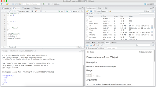
(點這裡看放大圖片)
?
查詢功能或檔案
Ex: ?rm()
##查詢 rm() 是什麼功能,解釋會出現在 Help 的視窗(右下)。
help()
Ex: help("dim")
##查詢 dim() 是什麼功能,解釋會出現在 Help 的視窗(右下)。
If the name has special characters, we need to put it in quotes:
help("+")
?"+"
以上功能已寫在 R Script (R-basic),有興趣的可以下載來跑跑看。
沒有留言:
張貼留言
歡迎發表意見